Eddy Current (EC)

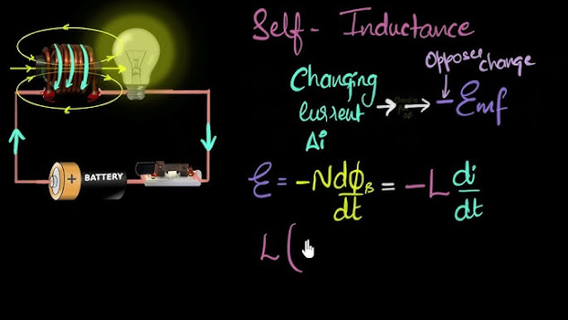
Eddy currents (EC) are induced electric currents that circulate in conductive materials when exposed to a changing magnetic field. In the context of magnetic resonance imaging (MRI) and transcranial magnetic stimulation (TMS), eddy currents play a significant role in influencing the magnetic field distribution and can have implications for image quality and stimulation accuracy. Here is an overview of eddy currents and their relevance in MRI and TMS:


1.      Generation of Eddy Currents:

o  MRI: In MRI, eddy currents are commonly generated when gradient coils rapidly switch magnetic field gradients during imaging sequences. These eddy currents arise due to Faraday's law of electromagnetic induction, where a changing magnetic field induces circulating currents in conductive structures, such as the MRI scanner components or the patient's body tissues.

o  TMS: In TMS, eddy currents can be induced in the brain tissue when the TMS coil generates a rapidly changing magnetic field to stimulate neural activity. These currents may affect the distribution and intensity of the magnetic field within the brain, influencing the efficacy and precision of TMS stimulation.

2.     Effects of Eddy Currents:

o  MRI Artifacts: Eddy currents in MRI systems can lead to image distortions, geometric distortions, and signal losses. These artifacts can impact the quality and accuracy of MRI images, affecting diagnostic interpretation and quantitative analyses.

o TMS Stimulation: In TMS, eddy currents can alter the spatial distribution of the magnetic field generated by the TMS coil, potentially leading to variations in the targeted brain region's stimulation intensity and depth. Understanding and mitigating eddy current effects are essential for ensuring consistent and reliable TMS outcomes.

3.     Mitigation Strategies:

o  MRI: To minimize eddy current artifacts in MRI, various techniques are employed, such as pre-emphasis gradients, gradient pre-emphasis, and active shimming. These methods help compensate for the effects of eddy currents and improve image quality.

oTMS: In TMS, coil design, orientation, and pulse waveform parameters can be optimized to reduce eddy current effects and enhance the precision of neural stimulation. Computational modeling and calibration techniques are also used to account for eddy current influences on TMS outcomes.

4.    Research and Development:

o  Ongoing research in MRI and TMS focuses on understanding the mechanisms of eddy currents, developing advanced correction algorithms, and optimizing hardware configurations to mitigate eddy current-related issues. By addressing eddy current challenges, researchers aim to enhance imaging accuracy, stimulation efficacy, and safety in clinical applications.

In summary, eddy currents are induced electric currents that arise in response to changing magnetic fields in MRI and TMS systems. Understanding the impact of eddy currents on image quality, stimulation accuracy, and safety is essential for optimizing imaging protocols and TMS procedures in research and clinical settings. Efforts to mitigate eddy current effects through technological advancements and methodological improvements contribute to the advancement of MRI and TMS techniques for neuroimaging and neuromodulation applications.


Comments

Popular posts from this blog

Relation of Model Complexity to Dataset Size

Core Concept The relationship between model complexity and dataset size is fundamental in supervised learning, affecting how well a model can learn and generalize. Model complexity refers to the capacity or flexibility of the model to fit a wide variety of functions. Dataset size refers to the number and diversity of training samples available for learning. Key Points 1. Larger Datasets Allow for More Complex Models When your dataset contains more varied data points , you can afford to use more complex models without overfitting. More data points mean more information and variety, enabling the model to learn detailed patterns without fitting noise. Quote from the book: "Relation of Model Complexity to Dataset Size. It’s important to note that model complexity is intimately tied to the variation of inputs contained in your training dataset: the larger variety of data points your dataset contains, the more complex a model you can use without overfitting....

Linear Models

1. What are Linear Models? Linear models are a class of models that make predictions using a linear function of the input features. The prediction is computed as a weighted sum of the input features plus a bias term. They have been extensively studied over more than a century and remain widely used due to their simplicity, interpretability, and effectiveness in many scenarios. 2. Mathematical Formulation For regression , the general form of a linear model's prediction is: y^ ​ = w0 ​ x0 ​ + w1 ​ x1 ​ + … + wp ​ xp ​ + b where; y^ ​ is the predicted output, xi ​ is the i-th input feature, wi ​ is the learned weight coefficient for feature xi ​ , b is the intercept (bias term), p is the number of features. In vector form: y^ ​ = wTx + b where w = ( w0 ​ , w1 ​ , ... , wp ​ ) and x = ( x0 ​ , x1 ​ , ... , xp ​ ) . 3. Interpretation and Intuition The prediction is a linear combination of features — each feature contributes prop...

Predicting Probabilities

1. What is Predicting Probabilities? The predict_proba method estimates the probability that a given input belongs to each class. It returns values in the range [0, 1] , representing the model's confidence as probabilities. The sum of predicted probabilities across all classes for a sample is always 1 (i.e., they form a valid probability distribution). 2. Output Shape of predict_proba For binary classification , the shape of the output is (n_samples, 2) : Column 0: Probability of the sample belonging to the negative class. Column 1: Probability of the sample belonging to the positive class. For multiclass classification , the shape is (n_samples, n_classes) , with each column corresponding to the probability of the sample belonging to that class. 3. Interpretation of predict_proba Output The probability reflects how confidently the model believes a data point belongs to each class. For example, in ...

Supervised Learning

What is Supervised Learning? ·     Definition: Supervised learning involves training a model on a labeled dataset, where the input data (features) are paired with the correct output (labels). The model learns to map inputs to outputs and can predict labels for unseen input data. ·     Goal: To learn a function that generalizes well from training data to accurately predict labels for new data. ·          Types: ·          Classification: Predicting categorical labels (e.g., classifying iris flowers into species). ·          Regression: Predicting continuous values (e.g., predicting house prices). Key Concepts: ·     Generalization: The ability of a model to perform well on previously unseen data, not just the training data. ·         Overfitting and Underfitting: ·    ...

Kernelized Support Vector Machines

1. Introduction to SVMs Support Vector Machines (SVMs) are supervised learning algorithms primarily used for classification (and regression with SVR). They aim to find the optimal separating hyperplane that maximizes the margin between classes for linearly separable data. Basic (linear) SVMs operate in the original feature space, producing linear decision boundaries. 2. Limitations of Linear SVMs Linear SVMs have limited flexibility as their decision boundaries are hyperplanes. Many real-world problems require more complex, non-linear decision boundaries that linear SVM cannot provide. 3. Kernel Trick: Overcoming Non-linearity To allow non-linear decision boundaries, SVMs exploit the kernel trick . The kernel trick implicitly maps input data into a higher-dimensional feature space where linear separation might be possible, without explicitly performing the costly mapping . How the Kernel Trick Works: Instead of computing ...